What follows is an introduction to the harmonic oscillator, as a complement of the fourth exercise, third lesson, of Leonard Susskind’s The Theoretical Minimum: Classical Mechanics book.
If you’re interested in solutions to other exercises, you may want to head here.
Note: This article has been generated from .tex files by Pandoc. Pandoc works reasonably well, but tackles a sophisticated problem, full of corner cases; I’ve tried to fix a few issues, but for instance, references to labels are broken. If that really bothers you, you can still read the .pdf.
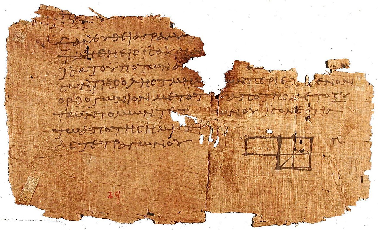
Oxyrhynchus papyrus (P.Oxy. I 29) showing fragment of Euclid’s Elements through math.ubc.ca wikimedia.org – Public domain
Exercise 1. Show by differentiation that the general solution to Eq. \((6)\) is given in terms of two constants \(A\) and \(B\) by \[x(t) = A\cos\omega t + B\sin\omega t\] Determine the initial position and velocity at time \(t=0\) in terms of \(A\) and \(B\).
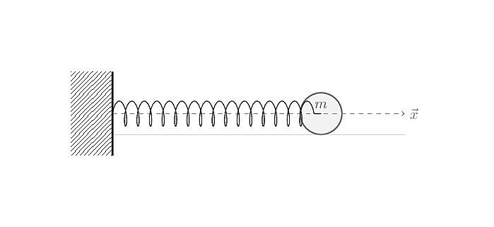
We’re in the case of a \(1\)-dimensional harmonic oscillator, depicted below as a mass \(m\) set on a frictionless ground attached to a fixed element to the left by a horizontally positioned spring of constant \(k\).
Remark 1. Almost equivalently, we could have
worked in a vertical setting, which, on one hand, would have avoided us
the need for a frictionless ground, but on the other hand, would make
the equation slightly more complicated.
There are interesting, complementary aspects to both cases. Because the
differences are minute, we can explore both of them here.
Harmonic oscillators play a major role in physics, as explained by Feynman in Chapter \(21\) of the first volume of his Lectures on Physics:
The harmonic oscillator, which we are about to study, has close analogs in many other fields; although we start with a mechanical example of a weight on a spring, or a pendulum with a small swing, or certain other mechanical devices, we are really studying a certain differential equation. This equation appears again and again in physics and in other sciences, and in fact it is a part of so many phenomena that its close study is well worth our while.
Some of the phenomena involving this equation are the oscillations of a mass on a spring; the oscillations of charge flowing back and forth in an electrical circuit; the vibrations of a tuning fork which is generating sound waves; the analogous vibrations of the electrons in an atom, which generate light waves; the equations for the operation of a servosystem, such as a thermostat trying to adjust a temperature; complicated interactions in chemical reactions; the growth of a colony of bacteria in interaction with the food supply and the poisons the bacteria produce; foxes eating rabbits eating grass, and so on; all these phenomena follow equations which are very similar to one another, and this is the reason why we study the mechanical oscillator in such detail.
Thus, we’ll take the time to analyze it more precisely than what is
expected here: this is the occasion to present some aspects not covered,
or not covered as explicitly in the book.
Despite everything happening in one-dimension, we’ll use a vector
position \(\pmb{x}\), which is a
function of time. Hence, the vectors for speed and acceleration will
respectively be \(\pmb{v}=\dot{\pmb{x}} =
\dfrac{d}{dt}\pmb{x}(t)\) and \(\pmb{a}=\ddot{\pmb{x}} =
\dfrac{d^2}{dt^2}\pmb{x}(t)\). Note that we’re representing
vectors with bold font instead of arrows; bold font is rather common in
physics. This should be the only additional thing needed to follow
through for someone having read the book up to this stage.
Contact force, normal force, friction force
The contact
force is the force resulting from the contact of two objects. It is
generally decomposed into vertical and horizontal components. The
horizontal component perhaps is the most intuitive: it corresponds to friction forces. For
instance, after having given a gentle push to an object an on ordinary
table, it will only move up to a certain point: it is progressively
stopped by the friction between the object and the table. You may think
that this friction is caused at least in part because at a microscopic
scale, both the object and the surface are far, far from being perfectly
plane, and even more so at an atomic scale.
But this is false. As a counter-example, consider gauge blocks,
manufactured to be extremely flat: their surfaces, far from being
frictionless to each other, cling!
Because a rigorous understanding of friction forces requires advanced
mechanics knowledge, we can satisfy ourselves with Feynman’s
vulgarization, from Chapter \(12\) of the first volume of his
Lectures on Physics:
There is another kind of friction, called dry friction or sliding friction, which occurs when one solid body slides on another. In this case a force is needed to maintain motion. This is called a frictional force, and its origin, also, is a very complicated matter. Both surfaces of contact are irregular, on an atomic level. There are many points of contact where the atoms seem to cling together, and then, as the sliding body is pulled along, the atoms snap apart and vibration ensues; something like that has to happen. Formerly the mechanism of this friction was thought to be very simple, that the surfaces were merely full of irregularities and the friction originated in lifting the slider over the bumps; but this cannot be, for there is no loss of energy in that process, whereas power is in fact consumed. The mechanism of power loss is that as the slider snaps over the bumps, the bumps deform and then generate waves and atomic motions and, after a while, heat, in the two bodies.
[...]
It was pointed out above that attempts to measure \(\mu\) by sliding pure substances such as copper on copper will lead to spurious results, because the surfaces in contact are not pure copper, but are mixtures of oxides and other impurities. If we try to get absolutely pure copper, if we clean and polish the surfaces, outgas the materials in a vacuum, and take every conceivable precaution, we still do not get \(\mu\). For if we tilt the apparatus even to a vertical position, the slider will not fall off—the two pieces of copper stick together! The coefficient \(\mu\), which is ordinarily less than unity for reasonably hard surfaces, becomes several times unity! The reason for this unexpected behavior is that when the atoms in contact are all of the same kind, there is no way for the atoms to “know” that they are in different pieces of copper. When there are other atoms, in the oxides and greases and more complicated thin surface layers of contaminants in between, the atoms “know” when they are not on the same part. When we consider that it is forces between atoms that hold the copper together as a solid, it should become clear that it is impossible to get the right coefficient of friction for pure metals.
The normal force is the vertical component of the contact force. An object on a table is affected by the Earth gravity, but naturally resists going through the table, unless of course, the object is really massive and/or the table very weak. There’s a bunch of complicated interactions at the atomic level from which this situation occurs: at a macroscopic scale, we simplify things and wrap this complexity by abstracting it as a (macroscopic) force.
Remark 2. In the case of the vertical setup, with a mass attached to a vertical spring, the mass is not in contact with a ground surface, so there would have been no need to discuss contact forces.
Remark 3. A static object on a flat surface corresponds to a special case where the horizontal component of the contact force (friction) is null. Hence, the contact force and the normal force are, in such a special case, one and the same. The exact same thing would happen in the case of a frictionless surface.
Newton’s laws
Let us start by recalling Newton’s
laws of motion:
Principle of inertia: Every body continues in its state of rest, or of uniform motion in a straight line, unless it is compelled to change that state by forces impressed upon it;
"\(\pmb{F} = m\pmb{a}\)": The change of motion [momentum] of an object is proportional to the force impressed; and is made in the direction of the straight line in which the force is impressed;
"action \(\Rightarrow\) reaction": To every action there is always opposed an equal reaction; or, the mutual actions of two bodies upon each other are always equal, and directed to contrary parts.
Remark 4. A force always is applied from an object, to another object; with the restriction that an object cannot apply a force to itself.
Remark 5. The second law is a actually a statement about momentum, from which we can derive \(\pmb{F}=m\pmb{a}\). More precisely, the momentum, called "motion" by Newton, is defined as \(\pmb{p} = m\pmb{v}\), which literally captures the idea of the speed \(\pmb{v}\) of a certain amount of matter \(m\). Then, it follows that the general case, \(\pmb{p}\) is as \(\pmb{v}\) a function of time.
The "change of motion" then refers to an infinitesimal change of the momentum over time, mathematically captured by the time derivative \(\dfrac{d}{dt}\pmb{p}\). The law can then be progressively written, assuming the mass \(m\) is constant over time: \[\pmb{F} = \frac{d}{dt}\pmb{p} = \frac{d}{dt}m\pmb{v} = m\frac{d}{dt}\pmb{v} = m\pmb{a}\,\boxed{\,}\]
Remark 6. It may seem weird to mention in the
previous Remark \(\ref{rem:L03E04:fma}\) that we assume the
mass \(m\) to be constant over time. In
the current context, this will be the case, but in general, likely
contrary to what any reasonable human would expect, they are exceptions.
More precisely, in special relativity, the mass is a function of the
velocity \(v\): \[m_{\text{rel}} =
\frac{m}{\sqrt{1-\dfrac{v^2}{c^2}}}\] We won’t delve into the
details here, but note that if \(v=\lVert
\pmb{v} \rVert\) is much smaller that \(c\), the speed of light, then the relative
mass \(m_{\text{rel}}\) and \(m\) are very close.
To say it otherwise, this assumption doesn’t hold at high
velocities.
Remark 7. In the second law, the force impressed
("\(\pmb{F}\)") is actually the force
resulting from all the other forced applied to an object, \(\sum_i\pmb{F}_i\), which is sometimes
called \(\pmb{F}_\text{net}\).
For instance, if you push a cart, \(\pmb{F}_\text{net}\) should contain at
least the force you are exerting, the gravity exerted by Earth, and the
contact force generated by the ground on the cart’s wheel. The sum of
all the forces applied to the cart that will ultimately
influence its motion.
As a result, in practice, when analyzing a situation so as to establish
the equation of motion of an object, one should start by identifying all
the external forces applied to this object.
Remark 8. A common special case of the second
law is to consider objects that, within a certain frame of reference, do
not move. Hence, by definition, their speed \(\pmb{v}\) would be \(0\), and so would be their acceleration.
That is, \(\sum_i\pmb{F}_i =
\pmb{0}\).
Another special case for the second law is when things move at constant
speed. Again, the acceleration would then be \(\pmb{0}\) and thus still \(\sum_i\pmb{F}_i = \pmb{0}\).
Remark 9. It is interesting to spend a moment
to ponder what the mass \(m\) of an
object really "is". Intuitively, for a non-physicist mass is another
word for weight, but not to a physicist.
Instead, in the context of the second law, physicists will observe that
the more mass there is, the more force will be needed to accelerate an
object. Conversely, the less mass there is, the less force will be
needed to alter the motion of an object. Thus, they would conceptualize
the mass as a measure of resistance to acceleration
(change of movement).
This is the second time we meet a subtlety regarding masses, the first
one being Remark \(\ref{rem:L03E04:relmass}\) about how mass
is a function of the velocity. We’ll come back later once again in a
moment at some more subtlety regarding mass.
Remark 10. In the case of a static object laying
on a flat surface, one may think that the gravitational force exerted by
the Earth on the object and the normal force/contact force arising from
the contact of the object with the surface are two opposite forces, in
the sense of Newton’s third law: after all, they are indeed of equal
intensity and opposite directions.
But this is incorrect: in such a situation, we actually have
two pairs of opposite forces, in the sense of Newton’s third
law:
\(\pmb{F}_{o,e}\) and \(\pmb{F}_{e,o}\), respectively the gravitational force exerted by the object on Earth, and the gravitational force exerted by Earth on the object;
\(\pmb{F}_{o,t}\) and \(\pmb{F}_{t,o}\), respectively the contact force exerted by the object on the table, and the contact force exerted by the table on the object.
Now to be more complete, there’s even a third pair of forces,
which would be in almost all practical situations negligible, namely,
the gravitational forces exerted by the surface on the object, and by
the object on the surface.
A good exercise to check one understanding of this topic would be to try
to identify forces in the case of a hand pressed on a (static) wall, or
in the case of two hands pressed against each other.
Remark 11. Newton’s third law is actually a
consequence of the principle of conservation
of momentum: essentially, in a closed system, the total momentum is
a constant over time.
This is a key idea in modern physics, and will be key later in the
book.
Hooke’s law
Hooke’s law,
as Newton’s laws, is an empirical law, that is, which has been
found by repeated experimentation. Essentially, it states that the force
needed to extend or compress a spring by a given distance varies
linearly with the distance during which the spring is
extended/compressed. That linear factor \(k\) is the spring’s constant. This
force is thus a function of that distance/displacement \(\pmb{\delta}\): \[\pmb{F}_s(\pmb{\delta}) = k \pmb{\delta}\]
The equation could be read as something like:
If I don’t compress/stretch the spring (\(\pmb{\delta}=\pmb{0}\)), no force is exerted;
The more I compress/stretch the spring, the greater the force, where the relation between both varies linearly.
Remark 12. In most practical cases, \(\pmb{\delta}\) will be a function of time \(\pmb{\delta}(t)\); thus, the force itself will be a function of time: \(\pmb{F}_s(\pmb{\delta}(t))\).
Remark 13. By Newton’s third law, if there’s an object exerting a force on the spring, then the spring also exerts a force on the object, of equal intensity, but in the opposite direction. Hence, equivalently, Hooke’s law could be reformulated in the form presented in the book: \[\pmb{F}_s(\pmb{\delta}) = - k \pmb{\delta}\]
Remark 14. You may sometimes find that last
version of the law, as is the case in the book, written as \(\pmb{F}_s(\pmb{x}) = -k\pmb{x}\). This is a
convenient choice that physicists can make, where, by identifying the
origin of the coordinate system as the rest position of the mass, the
measure of displacement \(\pmb{\delta}\) will indeed always match the
position vector \(\pmb{x}\).
This can be summarized by saying that \(bm{F}_s\) is the the force pulling the mass
back to its rest position.
Remark 15. If you have a spring or two around (architect lamps are a good source) and some regular weight (small tableware, such as iron tea cups would do), you should be able to easily verify this law experimentally. In this case, the objects’ weight will be the source of a gravitational force (we’ll come back to the gravitational force in a moment): doubling the mass (attaching two cups) should double the deformation of the spring.
Remark 16. Were you at least to imagine the previous experiment, you would realize that there must so some limits to this law: the spring could break or be irremediably deformed. Hooke’s law is actually a first-order linear approximation, that works reasonably well in plenty of practical cases. There are more advanced models who generalize Hooke’s law, but they are of no use to us in this context.
Forces diagram
The goal of a force diagram, or a free body
diagram, is to identify the forces acting on an object, with the
intent of applying Newton’s second law, so as to later determine an
equation of movement for that object: we want to identify the sum of all
the forces acting on the object, \(\pmb{F}_\text{net}=\sum_i\pmb{F}_i\), who
are likely to contribute to the shape of its trajectory. Let’s complete
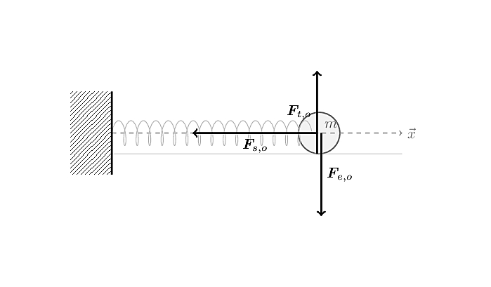
the diagram of our horizontal spring setup with:
- \(\pmb{F}_{e,o}\)
-
the gravitational force exerted by the earth on our object. Note that we haven’t talked about gravitation yet, and as you’ll see in a moment, we don’t need to, but this will be necessary for the vertical spring setup;
- \(\pmb{F}_{t,o}\)
-
the normal force exerted by the table on our object. Because the surface is frictionless, the normal force is the contact force;
- \(\pmb{F}_{s,o}\)
-
the force exerted by the spring on our object, which can be described by Hooke’s law.
Placement of the origin of the \(\vec{x}\)-axis As we’ve already
observed before, it can be interesting to identify the origin of our
coordinate system to the position where the system will be at
equilibrium/rest.
Intensities and signs Thanks the previous convention,
as discussed in Remark \(\ref{rem:L03E04:origin}\), Hooke’s law can
be used to determine the force exerted by the spring on the object, and
can be written as \(\pmb{F}_{s,o} =
-k\pmb{x}\).
We know, from Newton’s second law, that the contact/normal force exerted
by the table on the object is equal to \(-\pmb{F}_{o,t}\), where \(\pmb{F}_{o,t}\) is the force exerted by the
object on the table, which itself results from the gravitational force
\(\pmb{F}_{e,o}\), i.e. \[\pmb{F}_{t,o} = -\pmb{F}_{o,t} =
-\pmb{F}_{e,o}\]
As we’ll see quickly, we don’t actually need to compute anything
more, in this situation. We’ll nevertheless show how to compute the
gravitational force in the next section, when considering the similar
case of a mass attached to a vertical spring.
Applying Newton’s second law We can now use Newton’s
second law, \(\sum_i \pmb{F}_i = m\pmb{a} =
m\ddot{\pmb{x}}\) to deduce an equation of motion:
\[\begin{aligned} ~ && \pmb{F}_{e,o} + \pmb{F}_{t,o} + \pmb{F}_{s,o} &= m\ddot{\pmb{x}} \\ \Leftrightarrow && \pmb{F}_{e,o} - \pmb{F}_{e,o} + \pmb{F}_{s,o} &= m\ddot{\pmb{x}} \\ \Leftrightarrow && \pmb{F}_{s,o} &= m\ddot{\pmb{x}} \\ \Leftrightarrow && -k\pmb{x} &= m\ddot{\pmb{x}} \,\boxed{\,} \end{aligned}\]
Which is a second order, linear differential equation, homogeneous, with constant coefficients. It’s often rewritten, as is the case in the book, by defining \(\omega^2 = \dfrac{k}{m}\):
\[\boxed{\ddot{\pmb{x}} = -\omega^2\pmb{x}}\]
Gravitational force
To handle the case of a vertical spring, we won’t be able to brush the
gravitational force away as we did previously, and we’ll need to compute
it.
There are a few different ways to reach a formula for the gravitational
force, but perhaps the simplest one, in the context of studying a mass
attached to a vertical spring, would be to empirically study the fall of
an object of mass \(m\) in Earth’s
gravitational field.
One could proceed for instance by video-taping a vertically falling
object of known mass \(m\). The video
can then be discretized into a series of images, on which we could
measure the evolution of the position of the mass over time. From there,
we could compute the speed, as the variation of position, and the
acceleration, as the variation of speed.
Then, neglecting the air resistance (well, we could perform the
experiment in a vacuum), we can pretend
that there’s a single force acting on the mass, which is our
gravitational force.
The experiment could obviously be performed multiple times to improve
the accuracy. In the end, physicists have found that Earth’s gravity is
an acceleration vector \(\pmb{g}\) of
intensity \(9.81\,m.s^{-2}\), directed
towards the center of the Earth, which experimentally gives a
gravitational force of: \[\pmb{F}_{e,o} =
m\pmb{g}\]
Remark 17. A home-made reenactment of the
experiment would be difficult, especially if there’s a need for strong
precision, which would involve the presence of a vacuum. At least, more
difficult than experimentally validating Hooke’s law on a single
spring.
Historically, a simpler and more primitive setup was employed, for
instance by Galileo, which would involved measuring the speed of a ball
rolling on an inclined plane. A great way to lower the speed of the
"fall" and thus to get more accurate time measurements.
Remark 18. 1) Note that \(\pmb{g}\) captures not only the
gravitational force exerted by the Earth, but also captures the
contribution of the Earth’s rotation (centrifugal force).
2) Because the Earth is not a perfect sphere, the value of \(\lVert \pmb{g} \rVert\) is not uniform
everywhere on Earth; there are noticeable differences from city to city
for instance.
Remark 19. In Remark \(\ref{rem:L03E04:mass}\), we conceptualized
the mass as a measure of resistance to acceleration. Physicists call
this the inertial mass. And they conceptually distinguish it
from what they call the gravitational mass, which is the
property of matter that qualify how an object will interact with a
gravitational field.
We tacitly assumed that both are the same: this is the equivalence
principle, a cornerstone of modern theories of gravities. So far,
physicists haven’t been able to distinguish the two masses
experimentally either. But conceptually, they refer to two distinct
notions.
Mathematically, this means that in the case of a falling object subject
to a single force exerted by gravitation, by applying Newton’s second
law, we have: \[\begin{aligned}
~ && \pmb{F}_\text{net} = \pmb{F}_{e,o} &= m_i\pmb{a} \\
\Leftrightarrow && m_g\pmb{g} &= m_i\pmb{a} \\
\Leftrightarrow && \pmb{g} &= \pmb{a}
\end{aligned}\]
Remark 20. 1) Another approach could have been
to rely on Newton’s
law of universal gravitation. \[\pmb{F}_{e,o} = -G\frac{m_e m_o}{\lVert
\pmb{r}_{e,o} \rVert^2}\hat{\pmb{r}}_{e,o}\] But not only is this
law also empirical, but it would involve knowing the mass of the Earth
\(m_e\), the gravitational constant
\(G\), etc.
2) Similarly we could delve into Einstein’s
theory of general relativity, but the prerequisites would again have
been more sophisticated than exposing a basic experiment.
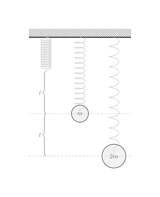
Vertical spring
We know have all we need to study a variant of our previous setup,
slightly more complicated mathematically, where a mass \(m\) is attached to the end side of a
vertical spring of constant \(k\),
itself firmly attached to a fixed element at its top:
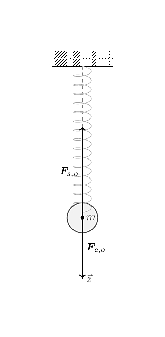
We’ll choose the same convention regarding the origin of our coordinate system (see Remark \(\ref{rem:L03E04:origin}\)). Contrary to the previous case, there’s no other force to counterbalance the gravitational force \(\pmb{F}_{e,o}\); applying Newton’s second law gives: \[\begin{aligned} ~ && \sum_i \pmb{F}_i = \pmb{F}_{e,o} + \pmb{F}_{s,o} &= m\ddot{\pmb{x}} \\ \Leftrightarrow && m\pmb{g} - k\pmb{x} &= m\ddot{\pmb{x}} \\ \Leftrightarrow && \ddot{\pmb{x}} &= -\omega^2\pmb{x}+\pmb{g} \end{aligned}\] Again, with \(\omega^2 = \dfrac{k}{m}\); so the only difference is that we get an additional constant \(\pmb{g}\), but this still is a second-order linear differential equation with constant coefficients.
Remark 21. However, this differential equation is said to be non-homogeneous because of the non-zero constant \(\pmb{g}\), by opposition with the previous homogeneous equation obtained from the horizontal spring setup.
Verifying the solution
Solving differential equations, mathematically, can be rather involved.
For such simple equations, mathematicians themselves may find it
sufficient to make an educated guess by tweaking an exponential-based
function, despite having explored the subject with much more
depth.
We won’t discuss the details here, and will pragmatically satisfy
ourselves with verifying that the proposed solution actually solves the
equation: \[x(t) = A\cos\omega t +
B\sin\omega t\]
Remark 22. We’ve been before expressing all our equations with vectors so far, but because we’re working in one-dimension, we can divide everything by \(\pmb{\hat{x}}\) and work from the resulting scalar equations.
And indeed, the proposed solution does solve the equation for the horizontal spring setup. \[\begin{aligned} \ddot x(t) &= -A\omega^2\cos\omega t - B\omega^2\sin\omega t \\ ~ &= -\omega^2 (A\cos\omega t + B\sin\omega t) \\ ~ &= -\omega^2 x(t) \,\boxed{\,} \end{aligned}\]
But it doesn’t solve the vertical setup; we’ll get there quickly, this isn’t much more complicated. You may want to try by yourself to see if you can tweak the solution of the homogeneous equation to solve the non-homogeneous one.
Initial conditions
Let’s start by computing the expression of the velocity: \[\dot x(t) = -A\omega\sin\omega t +
B\omega\cos\omega t\] Then, at \(t=0\), we have: \[\begin{aligned}
x(0) = && A\cos(0) + B\sin(0) &= \boxed{B} \\
\dot x(0) = && -A\omega\sin(0) + B\omega\cos(0) &=
\boxed{A\omega}\,\boxed{\,}
\end{aligned}\]
Equations and initial conditions for the vertical
setup
There are general mathematical methods for reaching a solution to a
non-homogeneous linear second-order differential equation with constant
coefficient from a homogeneous, but again, suffice for us to verify that
the following would work: \[x(t) =
A\cos\omega t + B\sin\omega t + \frac{g}{\omega^2}\] Indeed:
\[\begin{aligned}
\ddot x(t) &= -A\omega^2\cos\omega t - B\omega^2\sin\omega t \\
~ &= -A\omega^2\cos\omega t - B\omega^2\sin\omega t
-\frac{\omega^2}{\omega^2}g + g\\
~ &= -\omega^2 (A\cos\omega t + B\sin\omega t +
\frac{g}{\omega^2}) + g \\
~ &= -\omega^2 x(t) +g\,\boxed{\,}
\end{aligned}\] From there, we can again express the initial
position and speed as functions of \(A\) and \(B\), first by computing the expression of
the speed: \[\dot x(t) = -A\omega\sin\omega t
+ B\omega\cos\omega t\] And then by looking at what’s happening
at \(t=0\): \[\begin{aligned}
x(0) = && A\cos(0) + B\sin(0)+\frac{g}{\omega^2} &=
\boxed{B+\frac{g}{\omega^2}} \\
\dot x(0) = && -A\omega\sin(0) + B\omega\cos(0) &=
\boxed{A\omega}\,\boxed{\,}
\end{aligned}\]
Comments
By email, at mathieu.bivert chez: