On the (Real) Spectral Theorem

Proof. Let’s take a \(\pmb{v}\in V\). We assume \(V\) is not trivial, that is, \(V\) isn’t reduced to its zero vector \(\pmb{0}_V\), and so we can always choose \(\pmb{v} \neq \pmb{0}_V\)⁴.
Consider the following set of \(n+1\) vectors: \[\{ \pmb{v}, L(\pmb{v}), L^2(\pmb{v}), \ldots, L^n(\pmb{v}) \}\] where: \[L^0 := \text{id}_V;\qquad L^i := \underbrace{ L\circ L\circ\ldots\circ L }_{i\in\mathbb{N}\text{ times}}\] It’s a set of \(n+1\) vectors, but the space is \(n\) dimensional, so the vectors are not all linearly independent. This means there’s a set of \((\alpha_0, \alpha_1, \ldots, \alpha_n)\in\mathbb{C}^{n+1}\) which are not all zero, such that: \[\sum_{i=0}^n \alpha_iL^i(\pmb{v}) = \pmb{0}_V \label{qm:L03E01:not-linindep}\]

Here’s the "subtle" part. You remember what a polynomial is, something like: \[x^2 - 2x + 1\]

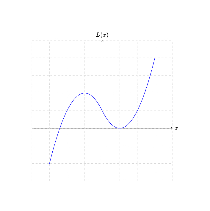
You know it’s customary to then consider this a function of a single variable \(x\), which for instance, can be a real number: \[L : \begin{pmatrix} \mathbb{R} & \rightarrow & \mathbb{R} \\ x & \mapsto & x^2 - 2x + 1 \\ \end{pmatrix}\] This allows you to graph the polynomial and so forth:

But that’s "kindergarten" polynomials so to speak. "Advanced" polynomials are not functions of a real variable. Rather, we say that \(L(x)\) or \(L\) is a polynomial of a single variable/indeterminate⁵ \(x\), where \(x\) stands for an abstract symbol.
The reason is that, when you say that \(x\) is a real number (or a complex number, or whatever), you tacitly assume that you can for instance add, subtract or multiply various occurrences of \(x\), but when mathematicians study polynomials, they want to do so without requiring additional (mathematical) structure on \(x\).
Hence, \(x\) is just a placeholder, an abstract symbol.
The set of polynomials of a single variable \(X\) with coefficient in a field \(\mathbb{F}\) is denoted \(\mathbb{F}[X]\). For instance, \(\mathbb{C}[f]\) is the set of all polynomials with complex coefficient of a single variable \(f\), say, \(P(f) = (3+2i)f^3 + 5f \in \mathbb{C}[f]\).
Now you’d tell me, wait a minute: if I have a \(P(X) = X^2 - 2X +1\), am I not then adding a polynomial \(X^2-2X\) with an element from the field, \(1\)?
Well, you’d be somehow right: the notation is ambiguous, in part inherited from the habits of kindergarten polynomials, in part because the context often makes things clear, and perhaps most importantly, because a truly unambiguous notation is unpractically verbose. Actually, \(X^2 - 2X +1\) is a shortcut notation for \(X^2 - 2X^1 +1 X^0\). So no: all the \(+\) here are between polynomials.
What does this mean that the \(+\) are between polynomials? Well, most often when you encounter \(\mathbb{F}[X]\), it’s actually a shortcut for \((\mathbb{F}[X], +_{\mathbb{F}[X]}, ._{\mathbb{F}[X]})\), which is a ring⁶ of polynomials of a single indeterminate over a field⁷ \(\mathbb{F}\). This means that \(X^2 - 2X +1\) is actually a shortcut for: \[1._{\mathbb{F}[X]}X^2 +_{\mathbb{F}[X]} (-2)._{\mathbb{F}[X]}X^1 +_{\mathbb{F}[X]} (1)._{\mathbb{F}[X]}X^0\]

Awful, right? Hence why we often use ambiguous notations and reasonable syntactical shortcuts.
The main takeaway though is that mathematicians have defined a set of precise rules (addition, scalar multiplication, exponentiation of an indeterminate), and that by cleverly combining such rules and only such rules, they have obtain a bunch of interesting results, and we want to use one of them in particular.
Let’s get back to our equation \((\ref{qm:L03E01:not-linindep})\); let me add some parenthesis for clarity: \[\sum_{i=0}^n \left(\alpha_iL^i(\pmb{v})\right) = \pmb{0}_V\]

Our goal is to transform this expression so that it involves a polynomial in \(\mathbb{C}[L]\)⁸.
Let’s start by pulling out the \(\pmb{v}\) on the left-hand side as such: \[\left(\underbrace{ \sum_{i=0}^n \alpha_iL^i }_{=:P(L)}\right)(\pmb{v}) = \pmb{0}_V\]

What’s \(P\) ? It’s a function which takes a linear operator on \(V\) and returns \(\ldots\) A polynomial? But then, we don’t know how to evaluate a polynomial on a vector \(\pmb{v}\in V\) so there’s an problem somewhere.
\(P\) actually returns a new linear operator on \(V\): \[P : \begin{pmatrix} (V \rightarrow V) & \rightarrow & (V \rightarrow V) \\ L & \mapsto & \sum_{i=0}^n \alpha_iL^i \\ \end{pmatrix}\]

But this means that while in (\(\ref{qm:L03E01:not-linindep}\)) the \(\sum\) was a sum of complex numbers, it’s now a sum of functions, and that \(\alpha_i L_i\) went from a multiplication between complex numbers to a scalar multiplication on a function.
The natural way, that is, the simplest consistent way, to do so, is to define them pointwise⁹ for two functions \(f, g : X \rightarrow Y\), we define \((f+g) : X \rightarrow Y\) by: \[(\forall x \in X),\ (f+g)(x) := f(x) + g(x)\] The process is similar for scalar multiplication: \[(\forall x \in X), (\forall y \in Y),\ (yf)(e) := yf(e)\]

We equip the space of (linear) functions (on \(V\)) with additional laws. All in all, \(P\) is well defined¹⁰, and that we can indeed pull the \(\pmb{v}\) out.
How then can we go from such a weird "meta" function \(P\) to a polynomial? Well, as we stated earlier, polynomials are defined by a set of specific rules: addition, scalar multiplication, and exponentiation of the indeterminate.
But if you look closely:

• Our point-wise addition has the same property as the additions on polynomial (symmetric, existence of inverse elements, neutral element, etc.)

• Similarly for our scalar multiplication;

• And our rules of exponentiation on function by repeated application also follows the rules of exponentiation for an indeterminate variable.

This mean that if we squint a little, if we only look at the expression \(P(L)\) as having nothing but those properties, then it behaves exactly as a polynomial. Hence, for all intents and purposes, it "is" a polynomial, and we can manipulate it as such.

So we can apply the fundamental theorem of algebra¹¹, we know that we can always factorize polynomials with complex coefficients as such: \[(\exists (c, \lambda_1, \ldots, \lambda_n)\in\mathbb{C}^{n+1}, c\neq 0),\ P(L) = c\prod_{i=0}^n (L-\lambda_i)\]

But don’t we have a problem here? \(L\) is an abstract symbol, and we’re "subtracting" it a scalar? Well, there are a few implicit elements: \[P(L) = c\prod_{i=0}^n (L^1 + (-\lambda_i)L^0)\]

Let’s replace this new expression for \(P(L)\) in our previous equation, which we can do essentially re-using our previous argument: the rules (addition, scalar multiplication, etc.) to manipulate polynomials are "locally" consistent with the rules to manipulate our (linear) functions: \[\left(c\prod_{i=0}^n (L^1-\lambda_i L^0)\right)(\pmb{v}) = \pmb{0}_V\]

Note that \(L^0\) becomes the identity function, and by using the previous point-wise operations, we can reduce it to: \[c\prod_{i=0}^n (L(\pmb{v})-\lambda_i\text{id}_V(\pmb{v})) = c\prod_{i=0}^n (L(\pmb{v})-\lambda_i\pmb{v}) = \pmb{0}_V\]

Now, \(c\neq 0\) by the fundamental theorem of algebra. So we must have: \[\prod_{i=0}^n (L(\pmb{v})-\lambda_i\pmb{v}) = \pmb{0}_V\]

Which implies that there’s at least a \(\lambda_j\) for which \[L(\pmb{v})-\lambda_j\pmb{v} = \pmb{0}_V \Leftrightarrow L(\pmb{v}) = \lambda_j\pmb{v}\]

But we’ve selected \(\pmb{v}\) to be non-zero: \(\lambda_j\) is then an eigenvalue \(\lambda_j\) associated to the eigenvector \(\pmb{v}\). ◻

Proof. I’m assuming that this is clear for you that the eigenvectors associated to the eigenvalues of a diagonalizable matrix makes a basis for the vector space. Again, refer to a linear algebra course for more.
Furthermore, you can refer to the book for a proof of orthogonality of the eigenvectors associated to distinct eigenvalues¹².
Note that I’ve included a mention to characterize the eigenvalues as real numbers: there’s already a proof in the book, but it comes with almost no effort with the present proof, so I’ve included it anyway.
Remains then to prove that the matrix representation \(M_H\) of \(H\) is diagonalizable (and that the eigenvalues are real). Let’s prove this by induction on the dimension of the vector space. If you’re not familiar with proofs by induction, the idea is as follow:

• Prove that the result is true, say, for \(n=1\);

• Then, prove that if the result is true for \(n=k\), then the result must be true for \(n=k+1\).

• If the two previous points hold, then you can combine them: if the first point hold then by applying the second point, the result must be true \(n=1+1=2\). But then by applying the second point again, it must be true that the result holds for \(n=2+1=3\).

• And so on: the result is true \(\forall n \in \mathbb{N}\backslash\{0\}\).

\(\boxed{n=1}\) Then, \(H\) is reduced to a \(1\times 1\) matrix, containing a single element \(h\). This is trivially diagonal already, and because \(H\) is assumed to be Hermitian, the only eigenvalue \(h = h^*\) is real.
\(\boxed{\text{Induction}}\) Assume the result holds for any Hermitian operator \(H : W \rightarrow W\) on a \(k\)-dimensional vector space \(W\) over \(\mathbb{C}\).
Let \(V\) be a \(k+1\)-dimensional vector space over \(\mathbb{C}\). By our previous lemma, \(H : V\rightarrow V\) must have at least one eigenvalue \(\lambda\in\mathbb{C}\) associated to an eigenvector \(\pmb{v}\in V\).
Pick \(\{\pmb{v}, \pmb{v}_2, \ldots, \pmb{v}_{k+1} \} \subset V\) so that \(\{\pmb{v}, \pmb{v}_2, \pmb{v}_3, \ldots, \pmb{v}_{k+1} \}\) is an (ordered) basis of \(V\)¹³.
Apply the Gram-Schmidt procedure¹⁴ to extract from it an (ordered) orthonormal basis \(\{ \pmb{b}_1, \pmb{b}_2, \ldots, \pmb{b}_{k+1} \}\) of \(V\); note that by construction: \[\pmb{b}_1 = \frac{\pmb{v}}{\lVert \pmb{v} \rVert}\]

That’s to say, \(\pmb{b}_1\) is still an eigenvector for \(\lambda\)¹⁵.
Now we’re trying to understand what’s the matrix representation \(D_H\) of \(H\), in this orthonormal basis. If you’ve taken the blue pill, you know how to "read" a matrix: \[D_H = \begin{pmatrix} \begin{pmatrix} \bigg\vert \\ H(\pmb{b}_1) \\ \bigg\vert \\ \end{pmatrix} & \begin{pmatrix} \bigg\vert \\ H(\pmb{b}_2) \\ \bigg\vert \\ \end{pmatrix} & \ldots & \begin{pmatrix} \bigg\vert \\ H(\pmb{b}_{k+1}) \\ \bigg\vert \\ \end{pmatrix} \end{pmatrix}\]

OK; let’s start by what we know: \(\pmb{b}_1\) is an eigenvector for \(H\) associated to \(\lambda\), meaning: \[H(\pmb{b_1}) = \lambda\pmb{b}_1 = \lambda\pmb{b}_1 + \sum_{i=2}^{k+1} 0 \times \pmb{b}_i = \begin{pmatrix} \lambda \\ 0 \\ \vdots \\ 0 \\ \end{pmatrix}\]

Rewrite \(D_H\) accordingly, and break it into blocks: \[D_H = \begin{pmatrix} \begin{matrix} \lambda \\ 0 \\ \vdots \\ 0 \end{matrix} & \begin{pmatrix} \bigg\vert \\ H(\pmb{b}_2) \\ \bigg\vert \\ \end{pmatrix} & \ldots & \begin{pmatrix} \bigg\vert \\ H(\pmb{b}_{k+1}) \\ \bigg\vert \\ \end{pmatrix} \end{pmatrix} = \begin{pmatrix}\begin{array}{c|c} \lambda & \qquad A \qquad\\ \hline 0 & \qquad ~ \qquad \\ \vdots & \qquad C \qquad \\ 0 & \qquad ~ \qquad \\ \end{array}\end{pmatrix}\]

Where A is a \(1\times k\) matrix (a row vector), and C a \(k\times k\) matrix. But then \(H\) is Hermitian, which means its matrix representation obeys: \[D_H = (D_H^T)^* = D_H^\dagger\]

This implies first that \(\lambda = \lambda^*\), i.e \(\lambda\) is real, and we’ll see shortly, can be considered an eigenvalue, as we can transform \(D_H\) in a diagonal matrix with \(\lambda\) on the diagonal.
Second, \(A^\dagger = (0\ 0\ \ldots\ 0) = A\), i.e: \[\begin{pmatrix}\begin{array}{c|c} \lambda & 0\quad\ldots\quad 0 \\ \hline 0 & \qquad ~ \qquad \\ \vdots & \qquad C \qquad \\ 0 & \qquad ~ \qquad \\ \end{array}\end{pmatrix}\]

Third, \(C = C^\dagger\). But then, C is a \(k\times k\) Hermitian matrix, corresponding to a Hermitian operator in a \(k\)-dimensional vector space. Using the induction assumption, it is diagonalizable, with real valued eigenvalues. Hence \(D_H\) is diagonalizable, and all its eigenvalues are real.
 ◻